Mechanism
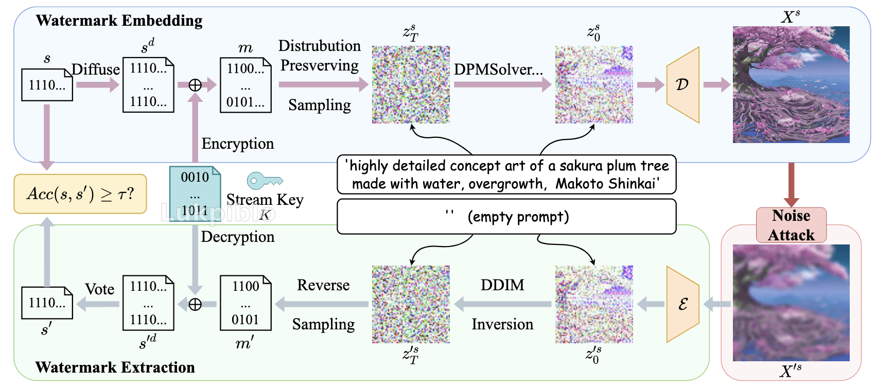
Watermark Diffusion
s : l × c f c × h f h w × w f h w → Diffuse s d : l × c × h × w \displaystyle{ s : l \times \frac{ c }{ f _{ c } } \times \frac{ h }{ f _{ h w } } \times \frac{ w }{ f _{ h w } } \xrightarrow[ ]{ \text{Diffuse} } s ^{ d } : l \times c \times h \times w } s : l × f c c × f h w h × f h w w Diffuse s d : l × c × h × w ( c × h × w ) \displaystyle{ \left( c \times h \times w \right) } ( c × h × w ) l \displaystyle{ l } l
Watermark randomization
m = s d ⊕ K ( e.g. ChaCha20 ) \displaystyle{ m = s ^{ d } \oplus K \left( \text{e.g. ChaCha20} \right) } m = s d ⊕ K ( e.g. ChaCha20 ) m ∼ U ( { 0 , 1 } ) \displaystyle{ m \sim U \left( \left\lbrace 0 , 1 \right\rbrace \right) } m ∼ U ( { 0 , 1 } )
Distribution-preserving sampling
Facts
y = dec ( m i j ) ∈ [ 0 , 2 l − 1 ] \displaystyle{ y = \text{dec} \left( m _{ i j } \right) \in \left[ 0 , 2 ^{ l } - 1 \right] } y = dec ( m ij ) ∈ [ 0 , 2 l − 1 ] m ∼ U ( { 0 , 1 } ) ⟹ y ∼ U ( { 0 , … , 2 l − 1 } ) ⟹ p ( y ) = 1 2 l \displaystyle{ m \sim U \left( \left\lbrace 0 , 1 \right\rbrace \right) \implies y \sim U \left( \left\lbrace 0 , \ldots , 2 ^{ l } - 1 \right\rbrace \right) \implies p \left( y \right) = \frac{ 1 }{ 2 ^{ l } } } m ∼ U ( { 0 , 1 } ) ⟹ y ∼ U ( { 0 , … , 2 l − 1 } ) ⟹ p ( y ) = 2 l 1
Notations
Let f ( x ) \displaystyle{ f \left( x \right) } f ( x ) N ( 0 , I ) \displaystyle{ \mathcal{ N } \left( 0 , I \right) } N ( 0 , I )
Let F ( x ) \displaystyle{ F \left( x \right) } F ( x ) N ( 0 , I ) \displaystyle{ \mathcal{ N } \left( 0 , I \right) } N ( 0 , I )
F − 1 ( x ) \displaystyle{ F ^{ - 1 } \left( x \right) } F − 1 ( x ) N ( 0 , I ) \displaystyle{ \mathcal{ N } \left( 0 , I \right) } N ( 0 , I )
Suppose z T s = g ( y ) \displaystyle{ z _{ T } ^{ s } = g \left( y \right) } z T s = g ( y )
Given
y ∼ U ( { 0 , 1 , … , 2 l − 1 } ) \displaystyle{ y \sim U \left( \left\lbrace 0 , 1 , \ldots , 2 ^{ l } - 1 \right\rbrace \right) } y ∼ U ( { 0 , 1 , … , 2 l − 1 } ) z T s ∼ N ( 0 , I ) \displaystyle{ z _{ T } ^{ s } \sim N \left( 0 , I \right) } z T s ∼ N ( 0 , I )
Review: Change of Variables Formula
x = g ( z ) ⟺ p X ( x ) = p Z ( z ) ∣ d z d x ∣ \displaystyle{ x = g \left( z \right) \iff p _{ X } \left( x \right) = p _{ Z } \left( z \right) \left| \frac{ {\text{d}z} }{ {\text{d}x} } \right| } x = g ( z ) ⟺ p X ( x ) = p Z ( z ) d x d z
Bridge y ∼ U \displaystyle{ y \sim U } y ∼ U z ∼ N \displaystyle{ z \sim \mathcal{ N } } z ∼ N
U \displaystyle{ U } U Dequantization & Normalizaion
Let y c = u + y 2 l , u ∼ N ( 0 , 1 ) \displaystyle{ y _{ c } = \frac{ u + y }{ 2 ^{ l } } , u \sim N \left( 0 , 1 \right) } y c = 2 l u + y , u ∼ N ( 0 , 1 )
y c ∼ U ( 0 , 2 l 2 l ) = U ( 0 , 1 ) \displaystyle{ y _{ c } \sim U \left( 0 , \frac{ 2 ^{ l } }{ 2 ^{ l } } \right) = U \left( 0 , 1 \right) } y c ∼ U ( 0 , 2 l 2 l ) = U ( 0 , 1 ) p Y c ( y c ) = 1 \displaystyle{ p _{ Y _{ c } } \left( y _{ c } \right) = 1 } p Y c ( y c ) = 1
p Z ( z ) = p Y c ( y c ) d y c d z ⟹ y c = ∫ p Z ( z ) d z = F Z ( z ) \displaystyle{ p _{ Z } \left( z \right) = p _{ Y _{ c } } \left( y _{ c } \right) \frac{ {\text{d}y} _{ c } }{ {\text{d}z} } \implies y _{ c } = \int p _{ Z } \left( z \right) {\text{d}z} = F _{ Z } \left( z \right) } p Z ( z ) = p Y c ( y c ) d z d y c ⟹ y c = ∫ p Z ( z ) d z = F Z ( z )
Thus.
Theorem (Inverse Transform Sampling)
z = F Z − 1 ( y c ) = F − 1 ( u + y 2 l ) i.e. z T s = ppf ( u + i 2 l ) \displaystyle{ z = F ^{ - 1 } _{ Z } \left( y _{ c } \right) = F ^{ - 1 } \left( \frac{ u + y }{ 2 ^{ l } } \right) \quad \text{i.e. } z _{ T } ^{ s } = \text{ppf} \left( \frac{ u + i }{ 2 ^{ l } } \right) } z = F Z − 1 ( y c ) = F − 1 ( 2 l u + y ) i.e. z T s = ppf ( 2 l u + i )
Extract the watermark from image:
y = ⌊ 2 l ⋅ F ( z T s ) ⌋ \displaystyle{ y = \left\lfloor 2 ^{ l } \cdot F \left( z _{ T } ^{ s } \right) \right\rfloor } y = ⌊ 2 l ⋅ F ( z T s ) ⌋ Equivilent: in a discretization view
y = i ⟺ z T s \displaystyle{ y = i \iff z _{ T } ^{ s } } y = i ⟺ z T s i \displaystyle{ i } i ( i 2 l , i + 1 2 l ] \displaystyle{ \left( \frac{ i }{ 2 ^{ l } } , \frac{ i + 1 }{ 2 ^{ l } } \right] } ( 2 l i , 2 l i + 1 ] f ( x ) \displaystyle{ f \left( x \right) } f ( x )
Reproduction
Implement --rotate distortion method
Set --num 500
Set --rotate 75 (aligned to Tree-Ring)
Discovery:
aligned with the results in the paper
robust to crop
sensitive to rotation
Transformation tpr_detection tpr_traceability mean_acc std_acc Median Blur 1.0 1.0 0.9987 0.0089 Resize 1.0 1.0 0.9961 0.0162 JPEG Compression 1.0 1.0 0.9884 0.0252 Gaussian Blur 1.0 1.0 0.9841 0.0246 Random Crop 1.0 1.0 0.9742 0.0164 Random Drop 1.0 0.99 0.9614 0.0373 Gaussian Std 1.0 1.0 0.9558 0.0594 Brightness 0.98 0.95 0.9532 0.0939 S&P Noise 1.0 0.98 0.9364 0.0664 ==Rotate (Our Discovery)== 0.0 0.0 0.5005 0.0335
Environment Configuration:
python 3.9
skimage==0.0 => scikit-image
transformers
huggingface_hub
Why Robust to Crop & Scale: Vote
Similar to voting, if the bit is set to 1 in more than half of the copies, the corresponding watermark bit is set to 1; otherwise, it is set to 0. This process restores the true binary watermark sequence s′.
假设图像被剪掉了 50%,这意味着有一半的水印副本丢失了。但由于 GS 在全图重复嵌入了多份副本,只要剩下的 50% 区域中,识别出的 Bit 1 比例依然占优(>1/2),根据上述的 Voting 规则,最终提取的原始比特流依然能被完美还原。
Why Sensitive to Rotation
旋轉徹底改變了所有塊的相對朝向和內部索引順序 。解碼器在 ( x , y ) \displaystyle{ \left( x , y \right) } ( x , y )
在 空域(Spatial Domain) 操作统计分布。
追求“分布不失真”(Performance-Lossless),这使得它必须深入到每一个具体的噪声采样点。这种对“点”的极致追求,牺牲了对几何变换(如旋转)的宏观鲁棒性。
频域的介入可以比较好地处理旋转